Tietokonejärjestelmän suorituskyky
Osaamistavoitteet: Materiaalissa esitetään erilaisia mittareita tietokonejärjestelmän suorituskyvyn mittaamiseen ja järjestelmien väliseen vertailuun.
Tässä materiaalissa esitetään tunnettuja metriikoita, määritelmiä ja standardeja, joiden avulla voidaan laskea vertailuarvoja eri tietokonejärjestelmien tai suorittimien vertailemiseksi.
Lähtökohtaisesti käyttäjänäkökulmasta tietokonejärjestelmän / suorittimen suorituskykyä mitataan ajan funktiona, ts. kauanko jonkun ohjelman/tehtävän suoritus kestää. Tällöin mitattavana on tietenkin kyseinen laskentatehtävän tyyppi, jota ajetaan eri järjestelmissä ja selvitetään mikä suoritin/järjestelmä selviytyy tällaisista tehtävistä nopeiten. Tässä suunnittelijoita ja ohjelmoijia sitten kiinnostaa, että mitkä laitteistokomponentit, tekniikat, käyttöjärjestelmän ja laiteohjelmiston toiminnallisuuksien toteutukset tai ohjelmistokomponentit osoittautuivat järjestelmässä pullonkauloiksi.
Yleisesti tietokonejärjestelmien / suorittimien vertailussa hyvä mittari, yllättäen, on kuinka paljon suoritusteho parani suhteessa aiempaan ratkaisuun, eli esimerkiksi montako käskyä suoritin suorittaa aikayksikössä tai mikä on muistin hakuaika. Tässä oleellista on valita vertailtaviin parametreihin sopiva mittari, koska erilaisia suorittimen ja sen toiminnan ohjauksen toteutuksia, jne, on varsin kirjavasti. Jo vertaillessa sekventiaalista suoritinta ja saman käskykannan toteuttavaa liukuhihnaversiota, todettiin että yksittäisen käskyn suoritusaika hieman piteni liukuhihnalla, mutta kokonaisuudessaan suoritusteho parani.
Amdahlin laki
Kuten todettiin, niin (käyttäjille) näkyvin suorituskyvyn parametri on ohjelmien suoritusaika ihmisten ajassa (Mittari 1). Nyt tietysti yleinen tapa kasvattaa tietokonejärjestelmän tehokkuutta on päivittää järjestelmäkomponentteja, esimerkiksi vaihdetaan suoritin tehokkaampaan, lisätään suorittimeen ytimiä rinnakkaislaskennan avuksi tai vaihdetaan muistipiirejä nopeampaan. Vaikka suorituskyky näin päivittämällä kasvaakin, saavutetun parannuksen mittaaminen ei ole ihan suoraviivaista.
Jo 60-luvulla esitettiin Amdahlin laki (kts. kuva sivulla), joka kuvaa miten järjestelmän osaresurssien kasvattaminen vaikuttaa ohjelman suoritusaikaan perustuen siihen miten päivitettyä resurssia suhteessa kokonaisaikaan käytetään.
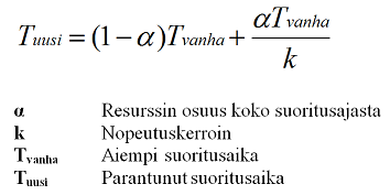
Esimerkki.
Tvanha = 100s, suoritusaika 100s
alfa = 0.6, eli resurssia käytetään 60% suoritusajasta
k = 3, resurssi lupaa kolminkertaisen nopeutus

Nyt parantunut suoritusaika on:
Tuusi = (1-0.6)*100s + (0.6*100s)/3 = 40s + 20s = 60s

Nyt suhteellinen nopeutus on Tvanha/Tuusi = 100s/60s = 1.67 -kertainen.
Havaitaan siis, että Amdahlin lain perusteella yksittäisen järjestelmäresurssin nopeuttaminen ei nopeuta koko järjestelmän toimintaa vastaavasti. Noh, tämä on aika maalaisjärkeen käypää, kun sen ajattelee esimerkiksi uusien osien hankkimisena mekaaniseen koneeseen. Jos uusi osa ei vaikuta järjestelmän pullonkaulaan, niin suoritustehon kasvu on marginaalinen.
Järjestelmän toimintanopeus
Toinen yleinen tapa nostaa suorituskykyä on parantaa järjestelmän toimintanopeutta. Nyt kun tietokonejärjestelmää ohjaa jokin kello / useita kelloja, saadaan kellojakson ajallisesta pituudesta yksikkö käskyjen/ohjelman suoritusajan mittaamiseen ja näin ollen toimintanopeuden arviointiin (Mittari 2).
Tässä
kellojakson ajallinen pituus = 1 / kellotaajuus (sekunteina). Saadaan ohjelman suoritukseen kulunut aika T = ohjelman kellojaksojen määrä * kellojakson pituus (sekunteina) tai vastaavasti kellotaajuuden avulla T = ohjelman kellojaksojen määrä / kellotaajuus.Suorittimien mikroarkkitehtuureissa tämä voisi tarkoittaa, että kellotaajuutta kasvatetaan (ylikellottamalla) tai käskykantaan toteutetaan CISC/RISC-käskyjä tai liukuhihnaan lisätään vaiheita ja/tai pilkotaan käskyjen suoritusta.
Käskyjen lukumäärä
Suoraviivainen tapa mitata ohjelman suoritusaikaa on laskea ohjelman (konekielisten) käskyjen määrä (Mittari 3).
Tämä mittari toki riippuu paljolti suorittimen käskykanta-arkkitehtuurista, paljonko rekistereitä on, miten muistiosoitukset tehdään, ovatko käskyt CISC- vai RISC-käskyjä, jne. Tietysti sekin vaikuttaa miten hyvin ohjelmoija ja kääntäjä ovat ohjelman toteutusta optimoineet valitulle suorittimelle.
Esimerkki. AMD K7-prosessorin konekielen käskyjen vaatimien mikrokoodin operaatioiden määrä (1-260) ja käskyn aiheuttama viive (1-200 kellojaksoa).
Käskyn suoritusaika
Aiempaa mittaria voidaan parantaa laskemalla kellojaksojen määrä käskyä kohti (engl. clock cycles per instruction, CPI) josta saadaan suorittimelle(/käskykannalle) yleisesti käskyn suoritukseen kuluva keskimääräinen aika (Mittari 4). Tietysti eri suorittimille käännetyn (saman) ohjelman käskyjen määrä ja CPI voivat olla hyvinkin erilaisia mikroarkkitehtuurin toteutuksesta riippuen. CPI on käypä mittari vertailemaan saman käskykannan toteuttavia suorittimia, esimerkkinä saman x86-käskykannan toteuttavat Intelin and AMD:n suorittimet. Mutta, jotta CPI olisi järkevä mittari, tulee keskimääräinen aika laskea erikseen eri tyyppisille käskyille kuten kokonaislukuoperaatiot, liukulukuoperaatiot, muistiosoitukset, ehdolliset käskyt, jne.
CPI:n avulla ohjelman suoritusaika T saadaan seuraavasti:
T = käskyjen lukumäärä * CPI * kellojakson aika.Esimerkki. Vertaillaan ohjelmia A ja B.
Suorittimen käskykannassa on määritelty kaksi CPI:tä erityyppisille käskyille:
Aritmeettiset operaatiot CPI = 1
Muistiosoitukset CPI = 8

Ohjelmissa käskyjä on seuraavasti:
A: ALU 12 + muisti 4 = 16 käskyä
B: ALU 6 + muisti 6 = 12 käskyä

A:n suoritusaika Ta = 12*1 + 4*8 = 44
B:n suoritusaika Tb = 6*1 + 6*8 = 54
Havaitaan, että ohjelmassa B oli lukumääräisesti vähemmän käskyjä, mutta A:n suoritusaika oli silti lyhyempi. Nyt vertailun tulos riippuisi siitä kumpaa parametria painotetaan käskyjen lukumäärää vai ohjelman suoritusaikaa?? Tästä syystä pelkkä CPI ei ole kattava mittari suorituskyvyn arvioimiseen.
Tietokonejärjestelmien vertailusta
Yleisesti tietokonejärjestelmissä yllä esitettyjä yksittäisiä mittareita/parametreja ei voida käyttää suorituskyvyn arviointiin tai vertailuun. Näin ollen käytetäänkin kaikkia yllä esitettyjä parametrejä suorituskyvyn arvioimiseen, eli saadaan kattavampi kuva, ja sitten myös vertailuun eri järjestelmien välillä:
| 1. | Ohjelman suoritukseen kulunut aika |
| 2. | Kellojakson pituus |
| 3. | Käskyjen lukumäärä ohjelmassa |
| 4. | CPI |
Yleisestä nopea
Nykyään tietokonejärjestelmät suunnitellaan yleiskäyttöisiksi työasemiksi (PC), joilla on lukematon määrä erilaisia käyttötarkoituksia. Tästä huolimatta suunnittelussa otetaan huomioon käyttäjien tarpeet, esimerkiksi nyt pelikoneissa panostetaan nopeaan grafiikkaan. Samoin laskentaservereissä, perustuen esimerkiksi GPU:hun, kannattaa miettiä millaisia laskentaoperaatioita yleisesti vaaditaan vaikkapa neuroverkko-pohjaisessa syväoppimisessa ja suunnitella suoritin vastaavasti. Kantava periaate suunnittelussa onkin tehdä yleisestä tapauksesta nopea (engl. "make the common case fast").
Okei.. no mikäs sitten olisi se yleinen tapaus?? Tätähän on vaikeaa, ellei mahdotonta määrittää. Tästä johtuen suorituskyvyn vertailuarvoja laskiessa (engl. benchmarking) käytetään joukkoa erilaisia (standardoituja) ohjelmia, jotka on suunniteltu yhdessä käytettäessä mittaamaan suorittimien tehokkuutta monipuolisesti. Esimerkiksi SPEC benchmarkit sisältävät kymmeniä erilaisia testiohjelmia, liukulukulaskennasta C-koodin kääntämisen kautta shakkipeliin, jne.
Esimerkki. Kuvassa SPEC-ohjelmat, joita käytettiin Intel Core i7-920 (2.66GHz) -suorittimen suorituskyvyn mittaamiseen.
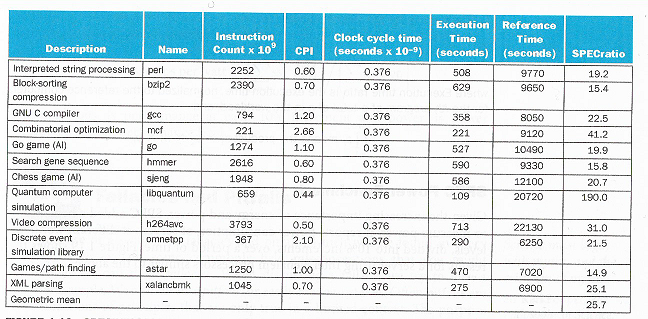
Huomataan, että eri testeistä ilmoitetaan eri ohjelmille kaikki neljä yllämainittua parametria: 1) ohjelman käskyjen määrä, 2) CPI, 3) kellonjakson pituus ja 4) ohjelman suoritusaika. Viimeinen parametri SPECratio on testit yhdistämällä saatu laskennallinen (normalisoitu) vertailuluku, joilla eri suorittimia voidaan verrata keskenään mainituissa testeissä.
Yleisiä benchmarkkeja
Muita yleisiä aiemmin ja nykyään käytettyjä benchmarkkeja ovat Whetstone, Dhrystone, Floating Point Operations per Second FLOPS.
Supertietokoneiden kanssa käytetään LINPACK vektorisuoritimille ja LAPACK, joka huomioi suorittimen sisäiset välimuistit vektorilaskennassa. HPCG benchmark arvioi myös I/O:n suorituskykyä muistin käytössä ja laskennan hajauttamisessa "reaalimaailman" sovelluksissa.
Kesäkuun 2020 supertietokoneiden TOP-500 listaus löytyy täältä. Kuten nähdään niin supertietokoneissa on nykyään jo useita miljoonia ytimiä.
Suomessa Tieteen Tietotekniikan keskuksen (CSC) laskentapalvelinkin pääsi kesällä 2017 sadan nopeimman supertietokoneen listalle. CSC on parhaillaan rakentamassa Kajaanin laskentakeskukseen uutta Lumi-supertietokonetta, josta halutaan kilpailukykyinen maailman nopeimpia supertietokoneita vastaan.
Tietokonejärjestelmien suunnittelun periaatteet
Kurssin toisen oppikirjan kirjoittaja David Patterson onkin esittänyt kahdeksan periaatetta tietokonejärjestelmien suunnitteluun:
- Ota huomioon Mooren laki. Ts. suunnittelijoiden pitäisi suunnitella tulevaisuutta varten, koska oletettavissa on, että mikropiirien resurssit kasvavat.
- Laitteiston ja ohjelmiston järjestelmäsuunnittelu kannattaa tehdä kerroksittain. Nyt kerroksilla (engl. abstraction layers) abstrahoidaan alempien kerrosten yksityiskohdat. Esimerkiksi sama käskykanta-arkkitehtuuri voidaan toteuttaa useilla eri mikroarkkitehtuureilla.
- Tee yleisestä tapauksesta nopea. Tämä on syytä huomioida jo käskykanta-arkkitehtuurin suunnittelussa.
- Laskennan rinnakkaisuus lisää suoritustehoa.
- Liukuhihnatoteutus lisää suoritustehoa.
- Ennustamalla lisää suoritustehoa. On keskimäärin nopeampaa arvata etukäteen ohjelman ehdollinen suoritus, kuin odottaa, että varmasti tiedetään miten ehdossa käy. Tämä seikka vaikuttaa jo siihen miten ohjelmat kannattaa toteuttaa konekielellä.
- Muistihierarkia nopeuttaa hitaan resurssin käyttöä.
- Redundanssi lisää toimintavarmuutta. Tietokonejärjestelmän komponentit, kuten kovalevyt tai muistipiirit, hajoavat varmasti ennenpitkää. Suunnittelussa on syytä varautua rinnakkaisilla peilatuilla resursseilla nostaen järjestelmän vikasietoisuutta. Esimerkkinä RAID-kovalevyt.
Anna palautetta
Kommentteja materiaalista?