HW4. Triangulation and Temporal Filtering
Due date: 2026-06-13 23:59.
Recommended Resources:
- SF: Sensing and Filtering, Steven M. LaValle, PDF
- Recorded Lectures and Slides
Part 1: Problems Using Visualizer
In the first part of the homework, you will explore trajectory filtering and spatial triangulation for a mobile robot using an interactive visualization tool. Rather than reasoning only analytically, you will observe how sets of sampled trajectories evolve over time under a motion model and how sensor measurements prune those sets via intersections of preimages.
State Space and Environment
The robot moves in a square planar environment:
E = [-1,1] \times [-1,1] \subset \mathbb{R}^2 .
\\\
The robot state includes position, heading, speed, and time:
(x_1, x_2, \theta, s, t) \in X, \quad
(x_1,
x_2)
\in E,
\\\
in which:
- 𝜃 ∈ 𝑆¹ is the heading (direction of motion),
- 𝑠 ≥ 0 is the speed along the heading.
Time
Time is discretized into measurement stages:
t \in \{0,1,2,3,4\}.
\\\
At each time stage:
- Starting from the sampled initial states at time 𝑡 = 0, trajectories are propagated forward using the motion model.
- Available sensor measurements at that time are applied to prune inconsistent trajectories.
- Only surviving trajectories are propagated into the next stage.
Initial Conditions
At time 𝑡 = 0, you may set up the initial conditions, resulting in the robot’s initial state being either known or partially/fully unknown. You may set up:
- Initial 𝑥₁ and 𝑥₂ values as
𝑥₁,₀and𝑥₂,₀. - Initial heading
𝜃₀. - Initial speed,
𝑠₀.
The visualization tool generates an initial set of states by sampling:
- positions (𝑥₁, 𝑥₂) on a uniform grid in 𝐸,
- headings 𝜃 from a finite set of angles,
- speeds 𝑠 from a finite set of values.
If no initial conditions are specified, the resulting samples represent complete uncertainty over the state space, and, therefore, over the possible trajectories. The visualizer only shows the (𝑥₁, 𝑥₂, 𝑡) projections of the trajectories. To visualize the paths that the robot executes, you need to further project the trajectories onto the (𝑥₁, 𝑥₂)-plane.
Motion Model
Each sampled state generates a candidate trajectory evolving over time. Between measurement stages, time can be further discretized into Δ𝑡 intervals, and each trajectory evolves according to:
\begin{bmatrix}
x_1 \\
x_2 \\
t
\end{bmatrix}_{k+1} =
\begin{bmatrix}
x_1 \\
x_2 \\
t
\end{bmatrix}_{k}
+
\begin{bmatrix}
𝑠_k \cos \theta_k \\
𝑠_k \sin \theta_k \\
1
\end{bmatrix}
\Delta t .
\\\
with optional bounded changes at each Δ𝑡 for:
- heading 𝜃,
- speed 𝑠.
Sensors
At each time stage, the following geometric sensors may report measurements.
1. Distance-to-Boundary Sensor
This nondeterministic sensor reports the distance from the robot’s position to the closest boundary of the environment:
h_1(x_1, x_2, \theta, 𝑠, t, d) = \min\{1 - |x_1|, 1 - |x_2|\} + 𝑑, \qquad 𝑑 ∈ [−\varepsilon_1, \varepsilon_1].
\\\
Geometrically, the preimage of this sensor is a thick band parallel to the boundary of the square.
2. Vertical 𝑥₁-Strip Sensor
This sensor constrains the 𝑥₁-coordinate:
h_2(x_1, x_2,\theta,𝑠,t,d) = x_1 + d, \qquad d \in [-\varepsilon_2,\varepsilon_2].
\\\
Its preimage is a vertical strip in the (𝑥₁, 𝑥₂)-plane.
3. Horizontal 𝑥₂-Strip Sensor
This sensor constrains the 𝑥₂-coordinate:
h_3(x_1, x_2,\theta,𝑠,t,d) = x_2 + d, \qquad d \in [-\varepsilon_3,\varepsilon_3].
\\\
The corresponding preimage is a horizontal strip in the (𝑥₁, 𝑥₂)-plane.
Triangulation and Trajectory Filtering
At a given time stage, any subset of sensors may be active.
Let the available measurements at a given time stage 𝑡 be denoted by 𝑦₁, 𝑦₂, and 𝑦₃, corresponding to sensors ℎ₁, ℎ₂, and ℎ₃, respectively. The set of states consistent with all available measurements is given by the intersection of the corresponding preimages:
\Delta(y_1, y_2, y_3) =
H_1^{-1}(y_{1})
\, \cap \,
H_2^{-1}(y_{2})
\, \cap \,
H_3^{-1}(y_{3}).
\\\
𝑃ₜ ⊆ E denotes the projection of consistent states at time 𝑡 onto position space. That is, 𝑃ₜ consists of all position pairs (𝑥₁, 𝑥₂) for which there exists a state with position (𝑥₁, 𝑥₂) that lies in the intersection of the preimages. Therefore, 𝑃ₜ represents the region in 𝐸 at time stage 𝑡 consistent with sensing.
A trajectory is kept at time stage 𝑡 if its position (𝑥₁(𝑡), 𝑥₂(𝑡)) lies in 𝑃ₜ. Trajectories that violate any measurement constraint are permanently discarded/filtered out.
Visualization
The visualization tool takes as input a set of parameters that define the initial conditions, sampling resolution, and motion model of the robot. These parameters determine which candidate trajectories are generated and how they evolve over time before being pruned by sensor measurements. The parameters are listed below:
Initial Conditions:𝑥₁,₀: Initial value of the robot’s 𝑥₁-position at time 𝑡 = 0 (if unspecified, all grid positions are used).𝑥₂,₀: Initial value of the robot’s 𝑥₂-position at time 𝑡 = 0 (if unspecified, all grid positions are used).𝜃₀: Initial heading angle at time 𝑡 = 0 (if unspecified, all sampled headings are used).𝑠₀: Initial speed at time 𝑡 = 0 (if unspecified, all sampled speeds are used).SamplingParameters:𝑥₁/𝑥₂ grid points: Number of grid points used to discretize the environment 𝐸 for initial position sampling.heading samples: Number of discrete heading values used to sample possible directions of motion.speed samples: Number of discrete speed values used to sample possible magnitudes of motion.𝑠ₘₐₓ: Maximum allowable speed used when sampling speeds and applying speed changes.Motion Model:time step, Δ𝑡: Time increment used to propagate trajectories between measurement stages.heading can change: Enables or disables random bounded changes in heading during propagation.speed can change: Enables or disables random bounded changes in speed during propagation.max heading change, Δ𝜃/Δ𝑡: Maximum change in heading allowed per time step when heading variation is enabled.max speed change, Δ𝑠/Δ𝑡: Maximum change in speed allowed per time step when speed variation is enabled.Measurements at time stages 𝑡 = {0, 1, 2, 3, 4}: For each time stage 𝑡, the following inputs may be provided:ℎ₁ (dist): Measurement reported by the distance-to-boundary sensor, specifying the robot’s distance to the closest boundary of the environment at time 𝑡.ℎ₂ (𝑥₁-strip): Measurement reported by the vertical strip sensor, constraining the robot’s 𝑥₁-coordinate at time 𝑡.ℎ₃ (x₂-strip): Measurement reported by the horizontal strip sensor, constraining the robot’s 𝑥₂-coordinate at time 𝑡.Measurement tolerancesfor each of the sensors can also be specified as 𝜀₁, 𝜀₂, and 𝜀₃.
Operating the Visualizer
Initialize: Resets the visualizer by resampling the initial set of trajectories at time 𝑡 = 0 using the current parameter values and clearing all previous propagation and pruning results.Next Stage (propagate + prune): Advances the motion model by one time stage by propagating all currently surviving trajectories forward in time and then removing any trajectories that violate the sensor constraints at the new stage, rendering:- a horizontal plane at the current time 𝑡.
- individual sensor preimages (faint colored regions).
- 𝑃ₜ, the projection of the intersection of all active preimages (highlighted region).
- surviving trajectories in (𝑥₁, 𝑥₂, 𝑡) space, such that (𝑥₁, 𝑥₂) ∈ 𝑃ₜ.
Run All: Automatically executes all remaining stages from the current time until the final stage, repeatedly applying propagation followed by pruning at each stage.Reset to Defaults: Restores all visualizer parameters to their default values but does not automatically resample trajectories or restart the simulation. To apply the restored defaults, the visualizer must be reinitialized using Initialize.Quit: Closes the visualization tool.
This helps visually interpret:
- which regions of space are consistent with the measurements.
- how sensing interacts with the motion model and dynamics.
- how triangulation emerges from intersecting geometric constraints.
- what paths the robot can execute in the environment, satisfying the initial conditions, motion model, and the sensor measurements.
Note: Any change to parameters—whether manual or via
Reset to Defaults — takes effect only after clicking Initialize.Part 2: Analytical Problems
Question 10
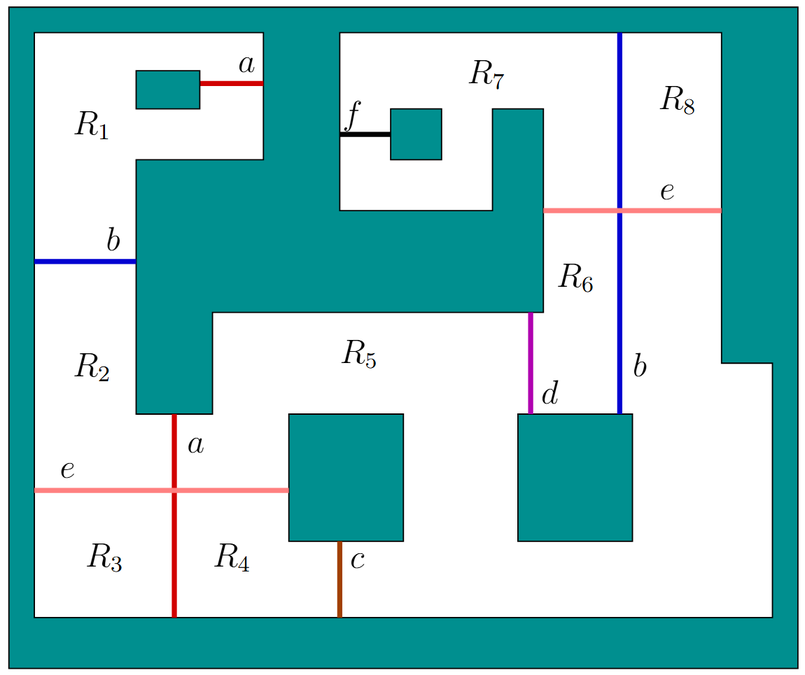
Consider the temporal filtering problem shown in the figure. An intruder, modeled as a point, moves around in a 2D environment 𝑋 = 𝐸. There are several beam detection sensors scattered around, each of which is a line segment that connects between two points on the boundary of 𝐸. If the intruder crosses a beam, then the letter that appears by the beam is the sensor observation. It is assumed that if the intruder touches a beam then it must cross it. Furthermore, it cannot touch exactly the intersection point between two beams. The environment 𝐸 contains eight regions, labeled from 𝑅₁ to 𝑅₈. Inside each region, the intruder may move freely without being detected.
Let 𝑿̃ be the set of all possible continuous intruder trajectories of the form 𝑥̃ : [0,100] → 𝐸, in which [0,100] is the time interval. Initially, it is unknown where in 𝐸 the intruder may be, other than assuming it is not placed directly on top of a beam at time 𝑡 = 0.
(5 correct statements)
Authors
Anna LaValle, Steven M. LaValle.
Anna palautetta
Leave your comments below: