Liukuhihnaprosessori
Osaamistavoitteet: Suorittimen liukuhihnatoteutuksen periaatteet sekä käskyjen ja datan riippuvuuksien aiheuttamista ongelmatilanteista selviäminen. Liukuhihnan suorituskyky.
Aiemmassa materiaalissa esittelimme sekventiaalisen suorittimen ja sen heikkouksia. Suorittimen toiminnan tehostamiseksi on esitetty osajärjestelmien liukuhihnoittamista (engl. pipeline), jossa kaikki osajärjestelmät ovat kokoajan aktiivisia suorittaen peräkkäisten käskyjen eri vaiheita. Kun käskyn suoritus etenee vaiheesta toiseen, sitä seuraava käsky tulee tilalle eli etenee nykyisen käskyn tilalle sen edelliseen vaiheeseen.
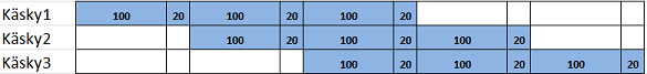
Kuvassa alla esimerkki liukuhihnasta y86-prosessorissa. Kirjaimet viittaavat käskyn suorituksen eri vaiheisiin: Fetch, Decode, Execute, Memory ja Write back. Huomataan ettei PC update-vaihetta enää ole, selitys tulee hetken päästä..
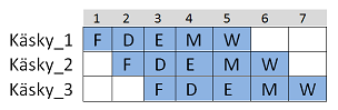
Näin liukuhihnasuorittimiessa käskyjen suorituksen suorituskyky/tehokkuus kasvaa, kun kellojakson pituuden määrittääkin pisimpään kestävän osajärjestelmän suoritusaika, eikä pisimmän käskyn koko suoritusaika. Kuvassa kolme käskyä (käsky_1 + käsky_2 + käsky_3) veisivät sekventiaalisessa prosessorissa 15 (3 x 5) aikayksikköä. Kuvan kaltaisella liukuhihnalla ne saadaan suoritetuksi jo 7:ssa aikayksikössä! Voidaan siis saavuttaa merkittävä parannus ohjelman suoritusaikaan.
Esimerkki. Vertaillaan
load word (lataa arvo muistista rekisteriin) käskyn suoritusta sekventiaalisessa ja liukuhihnoitetussa oikeassa MIPS-suorittimessa. 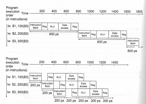
Liukuhihnalla siis kellojakson ajallinen pituus tippui neljäsosaan: 800ps -> 200ps. Nyt hyöty konkretisoituu siten, että suorittimesta saadaan käskyjen tuloksia ulos neljä kertaa nopeammin noin 200ps:n välein, kun taas sekventiaalisessa suorituksessa käskyn tuloksen saamiseen menee 800ps.
Mutta mutta..
Liukuhihnasuorittimissa on kuitenkin kaksi perustavanlaatuista ongelmaa. Ensiksi, sekventiaalisen suorittimen mikroarkkitehtuurissa eri osajärjestelmät käyttävät eri suorituksen vaiheissa sisäisiä rekistereitä ja signaaleita! Tästä seuraa liukuhihnatoteutuksissa ongelma, kun eri käskyt tarvitsisivat samoja sisäisiä rekistereitä suorituksen etenemiseen!
No, liukuhihnatoteutuksissa ongelma hoidetaan asettamalla vielä lisää sisäisiä, erillisiä, liukuhihnarekistereitä vaiheiden väliin. Näihin rekistereihin tallentuvat sitten käskyjen eri vaiheiden inputit ja outputit eli välitulokset seuraavat käskyä vaihe vaiheelta. Näin välitulokset eivät sotkeennu muiden käskyjen välituloksiin ja useaa eri käskyä voidaan suorittaa synkronoidusti samaan aikaan eri osajärjestelmissä. Tämän seurauksena toki jokaisen vaiheen suoritusaika pitenee hieman, mutta edelleen saadaan käskyjen tuloksia ulos nopeammassa tahdissa.
Toinen ongelma on se, että tietokoneohjelmien toimintalogiikka on (yleensä, heh heh) rakennettu siten, että ohjelman suoritus etenee käskystä seuraavalle järjestyksessä. Eli siis käskyn tulokset (outputit) ovat seuraavan käskyn argumentteja (inputit). Toisinsanoen, tämä tarkoittaa sitä, että käskyjen välillä on riippuvuuksia.
Jos katsotaan ym. kuvia, voidaan nähdä tilanteita, joissa edellisen käskyn tulokset eivät ole ehtineet Write back-vaiheeseen ennenkuin niitä tarvittaisiin seuraavan käskyn Decode-vaiheessa! Noh, ongelma hoidetaan tekemällä takaisinkytkentöjä vaiheiden välille siten, että välitulokset ovat seuraavien käskyjen käytössä ennenkuin ne on kirjoitettu tulosrekistereihin / muistiin.
Riippuvuusongelmia
Ok.. yllä esitetyt ongelmat näyttävät aika teoreettisilta, joten realisoidaanpas niitä esimerkkien ja niiden ratkaisujen avulla. Palataanpa mainittuihin riippuvuuksiin käskyjen välillä hieman tarkemmin:
- Riippuvuus käskyjen operadien välillä eli datahasardi (engl. data hazard). Esimerkiksi tällainen hasardi voi syntyä kun toisen käskyn output on toisen input.
- Riippuvuus käskyjen välillä eli ohjaus/kontrollihasardi (engl. control hazard). Esimerkkinä ehdolliset hyppykäskyt, joiden suoritus riippuu edellisen käskyn asettamista tilabiteistä.
(Ps. sanalle hasardi ei oikein löydy sopivaa suomennosta, joka ei kuulostaisi kömpelöltä..)
Datahasardi
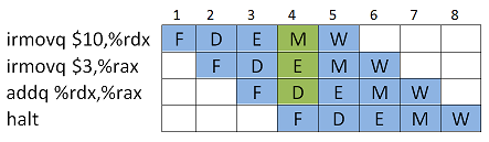
Tarkastellaan esimerkkikoodia, jossa ei sekventiaalisella prosessorilla suoritettaessa ole mitään ihmeellistä.
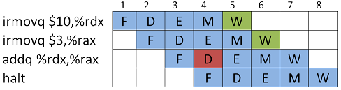
irmovq $10,%rdx  # rdx=10
irmovq $3,%rax   # rax=3
addq %rdx,%rax   # rax=rax+rdx
halt
Kun koodi ajetaan liukuhihnaprosessorissa, kohtaamme ongelman. Kaksi ensimmäistä käskyä eivät ehdi Write back-vaiheeseen (jossa niiden arvot kirjoitettaisiin kohderekistereihin), ennenkuin jo kolmas käsky tarvitsee niiden arvoja Decode-vaiheessaan.
Kuvassa nähdään, että rekisterien arvoja tarvittaisiin kellojaksolla 4, kun ne olisi saatavissa vasta kellojaksoilla 5 ja 6.
Data-hasardien selvittämiseksi on onneksi käytössä useita keinoja.
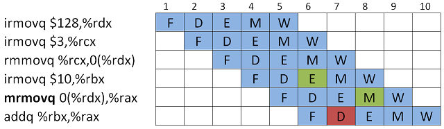
Viivyttäminen
Käskyn suoritusta voidaan viivyttää (engl. delay / stalling) lisäämällä väliin
nop-käskyjä, kunnes inputit ovat saatavilla. nop-käsky on tässä kätevä, koska se ei muuta suorittimen rekisterien sisältöjä mitenkään. 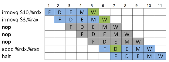
Kuvasta nähdään, että lisäämällä väliin 3 nop-käskyä, saadaan kahden aiemman käskyn Write Back-vaiheet suoritettua ennenkuin arvoja tarvitaan kolmannen käskyssä.
Toinen ratkaisutapa on että käskyt jäävät suorittamaan sen hetkistä vaihettaan, kunnes päästään etenemään. Tämä voidaan tehdä jäädyttämällä PC-rekisteri ja lisäämällä ohjelmaan väliin <bubble>ja jotka säilyttävät liukuhihnarekisterien arvot. Erona
nop-käskyyn on, ettei bubble välttämättä ole käsky. (Ok, usein bubble toteutetaan viemällä väliin nop-käskyjä..) 
Tässä inputit tarvittiin kellojaksolla 4, joten jäädytetään PC ja lisätään väliin bubble:ja alkaen kellojaksosta 5. Seurauksena on, että kaikki muutkin tätä seuraavat käskyt jäävät suorittamaan sen hetkistä vaihettaan, kunnes inputit saadaan Decode-vaiheeseen kellojaksolle 7.
Forwarding
Haittana aiemmissa keinoissa on, että lisäämällä väliin tyhjiä käskyjä tai "tyhjäkäynnillä" suorittimen suorituskyky ei ole optimaalinen, vaan kellojaksoja hukataan.
Forwarding (tai bypassing) pääsee ongelmasta eroon siten, että kontrollilogiikka yhdistää edellisten käskyjen välitulokset sisäisistä rekistereistä nykyisen käskyn inputteihin. Toisinsanoen, jos käskyn inputtia ei ole vielä saatavilla, tarkistetaan olisiko tulos jossain liukuhihnalla jo laskettu/noudettu.
Tämä keino on käytettävissä vain saman kellonjakson aikana tarjolla oleville signaaleille, josta syystä kellojakson suoritusaika hieman pitenee.
Kuvassa siis ensimmäisen ja toisen käskyn välitulokset (ikäänkuin liukuhihnan
valM ja valE) kellojaksosta 4 on kytketty addq-käskyn Decode-vaiheen input-signaaleiksi. Koska input-arvoja käytetään vasta addq:n Execute-vaiheessa, ne ehditään tässä kohti lukea. Muistiosoitushasardi
Kun käsky tekee muistiosoituksia hakeakseen inputin, rekisterikutsujen sijaan, voi syntyä load/use-hasardi, koska Memory-vaihe on vasta tulollaan, mutta muistista haettua arvoa tarvittaisiin jo seuraavassa käskyssä..
Nyt
addq-kutsulle ei saada asetettua molempia operandeja kellojaksossa 7. Neljännen käskyn (irmovq) output on jo saatavilla Execute-vaiheen jälkeen, mutta viidennen käskyn output saadaan vasta Memory-vaiheen jälkeen. Nyt ei voi käyttää Forwarding:ia, koska muistista rekisteriin lukeminen vaatii Memory-vaiheen ja näin molempien inputit on saatavilla vasta 8. kellojaksossa. Ratkaisu on yhdistää Viivyttäminen ja Forwarding. Eli lisätään bubble ja
addq-käsky suorittaa Decode-vaihettaan, kunnes molemmat inputit on saatavilla Forwarding:iä varten. 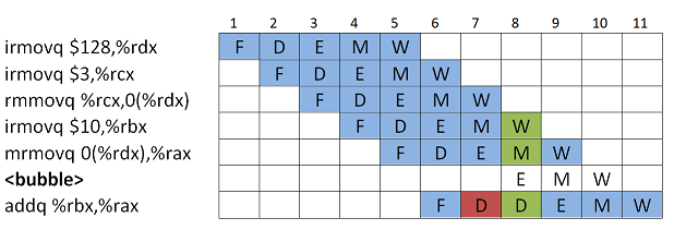
Ohjaushasardit
Ohjaus/kontrollihasardi (engl. control hazard) tarkoittaa sitä, että käskyjen välillä on riippuvuuksia siten, että käskyn tulos vaikuttaa siihen mistä ohjelman suoritusta jatketaan (engl. control dependency). Eli mikä onkaan seuraavan käskyn muistiosoite?
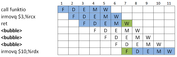
Aliohjelmahasardi
Tarkastellaan
ret-kutsusta johtuvaa mahdollista hasardia koodiesimerkin kautta.main:
call funktio
irmovq $10,%rdx
halt
funktio:
irmovq $3, %rcx
ret
Alla ohjelman suoritus liukuhihnalla. Nyt, aliohjelmaan hypätään ja se suoritetaan, mutta paluuosoite on tiedossa vasta
ret-käskyn Write back-vaiheessa. Siis, kun se on haettu pinosta (Memory-vaihe) ja talletettu PC-rekisteriin (Write back-vaihe).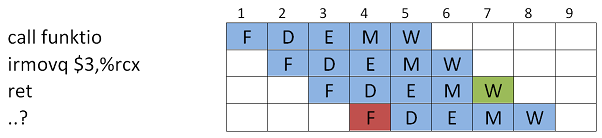
Ratkaisu tässäkin on lisätä väliin bubbleja, kunnes voidaan hyödyntää Forwarding:ia Fetch-vaiheeseen.
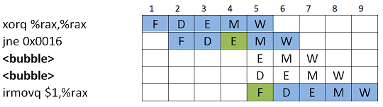
Ehdollinen hyppy
Ehdollinen hyppy voidaan liukuhihnasuorittimissa toteuttaa ennakoivasti kahdella tavalla: Ehdollinen hyppy toteutuu aina / Ehdollinen hyppy ei toteudu koskaan.
Ongelma ennustamisessa on, että riippuen ehdon tuloksesta, saatetaan oletuksena noutaa vääriä käskyjä, joskun tulos on eri kuin ennustettu.
Koodiesimerkki ehdollisesta hypystä y86:sessa.
0000: xorq %rax,%rax
0002: jne target         # Oletus: hyppy toteutuu aina!
000b: irmovq $1,%rax
0015: halt
0016: target:
0016:    irmovq $2,%rdx
0020:    irmovq $3,%rbx
002a:    ret
Ja koodin suoritus alla, nyt seuraavat (punaiset) käskyt on siis haettu oletuksen hyppy toteutuu aina mukaan. Oikea hyppyosoite selviää kuitenkin vasta käskyn Execute-vaiheessa.
Esimerkki. Kuvassa hyppykäskyn
jne 0x0016 kohdeosoitteesta on haettu liukuhihnalle etukäteen kaksi irmovq-käskyä. Mutta tilanne ei ole tässä suorittimessa mahdollinen, koska hyppyosoite selviää Execute-vaiheessa, koska siinä vaiheessa päivitetään tilaliput.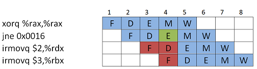
Ratkaisuna lisätään liukuhihnalle bubbleja, kunnes osoite on tiedossa.
Kuten myöhemmin tullaan näkemään, modernit suorittimet hakevat etukäteen käskyjä liukuhihnalle, jos tällöin ennustus ei toteudu, niin ratkaisuna on poistaa liukuhihnalta väärät käskyt ja lisätä väliin bubbleja.
Käskyjen ennakoiva uudelleenjärjestely
Joskus on mahdollista suorittimen (tai kääntäjän tai ohjelmoijan..) muokata tai muuttaa lennosta ohjelman suoritusta niin, että bubble:n tilalta suoritettaisiinkin myöhemmin tulossa olevia ohjelman käskyjä, jotka on tarkistettu ja todettu ettei niissö ei ole riippuvuuksia jumissa oleviin käskyihin.
Kuten arvata saattaa, tämä vaatiikin jo varsin edistynyttä ohjauslogiikkaa..
y86-liukuhihnatoteutus
Katsotaanpa seuraavaksi y86-64-suorittimen liukuhihnatoteusta ja miten siinä on ym. ongelmat hoidettu.
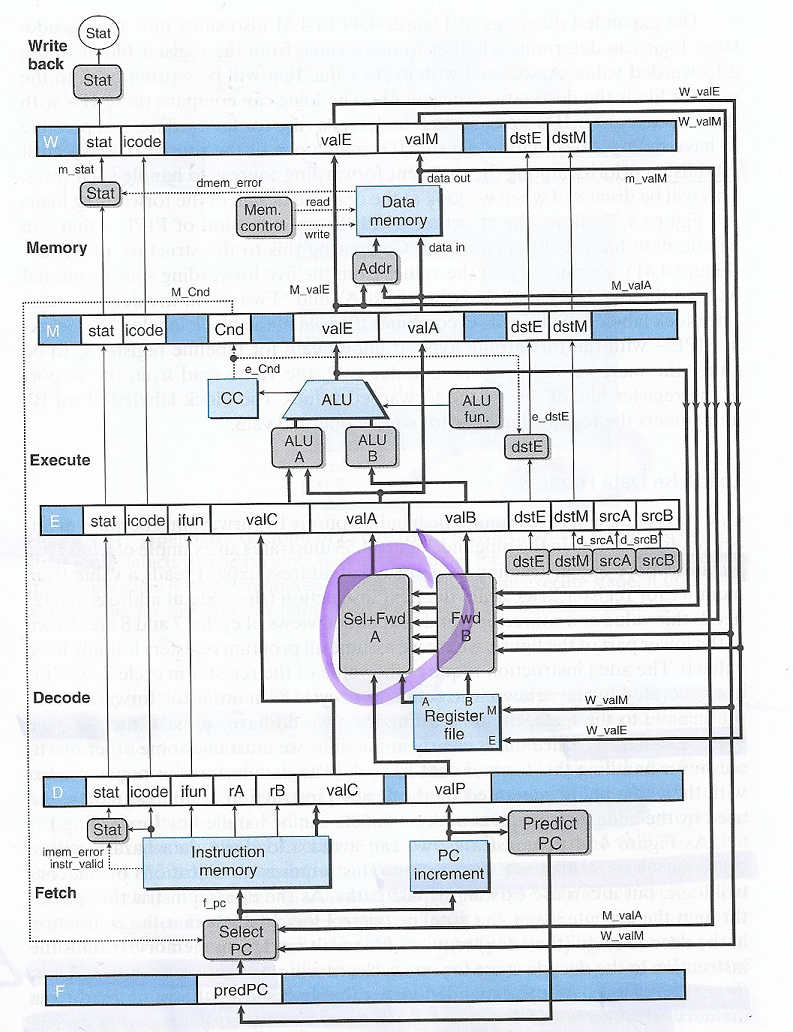
Nähdään, että toteutus (=mikroarkkitehtuuri) on monimutkaistunut huomattavasti. Ensinnäkin jokaisen vaiheen väliin on lisätty liukuhihnarekisterit (sininen väri). Lisäksi eri vaiheisiin on liitetty paljon lisää rekistereitä ja ohjaussignaaleja takaisinkytkennän toteuttamiseksi vaiheesta toiseen. Nyt Decode-vaiheessa on uusi ohjauslogiikkalohko (kuvassa ympyröity alue), joka valitsee joko nykyisen käskyn argumenteista tai muiden käskyjen välitulostuksista inputit nykyiselle käskylle.
Ok, mutta mistä tiedetään mikä näistä välitulostuksista valitaan milloinkin? y86-liukuhihnasuorittimessa on asetettu prioriteetti eri välituloksille ja sen mukaan valitaan argumentit käskystä jonka vaihe on lähinnä omaa vaihetta. Esimerkiksi, kun tarjolla ovat arvot edellisten käskyjen Execute- tai Memory-vaiheista, valitaan Execute-vaiheen käskyn välitulokset koska ne ovat lähinnä omaa vaihetta (Decode).
Lisäksi huomataan, että Fetch-vaiheeseen liitetty uusi ohjauslogiikka (Select PC) ja että PC Update-vaihe on kadonnut. Liukuhihnatoteutuksessa se siirretään Fetch-vaiheeseen, jotta seuraavan käskyn osoite haettaisiin mahdollisimman myöhään. Tämä lohko toteuttaa itseasiassa seuraaban käskyn muistiosoitteen ennustamista (engl. branch prediction) suorituskyvyn parantamiseksi. Tästä lisää myöhemmin..
Nyt Fetch-vaiheen liukuhihnarekisteri (Pred_PC) sisältää ennustetun seuraavan käskyn muistiosoitteen ao. sääntöjen pohjalta:
- Jos käsky ei ole ehdollinen tai hyppy, seuraavan käskyn osoite on nykyisen käskyn
valP:ssa - Jos käsky on ehdollinen, oletetaan että ehto toteutuu aina ja nyt rekisterissä on toteutumisen muistiosoite
- Jos ehto ei toteudu, seuraava osoite haetaan edellisen käskyn välitulostuksisa
valAtaivalMjoko Memory- tai Write Back-vaiheista
Liukuhihnan suorituskyky
Liukuhihnaprosessorin suorituskyvylle voimme esittää kaksi laskennallista parametriä:
- Suoritusaika/latenssi (engl. latency), joka kertoo käskyn/osajärjestelmän suoritusajan, yksikkö nykyään pikosekunti (ps)
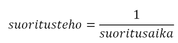
- Suoritusteho (engl. throughput), eli suoritettujen käskyjen määrä sekunnissa, yksikkö IPS (instructions per second)
Näiden avulla voimme laatia erilaisia liukuhihnaratkaisuja, joissa maksimoidaan suoritustehoa. Mikroarkkitehtuurissa voi suunnittelija jakaa käskyn suorituksen niin moneen vaiheeseen (teoriassa) kun on tarpeen ja viedä väliin niin monta liukuhihnarekisteriä kun tarvitaan. Itseasiassa moderneissa suoritintoteutuksissa esimerkiksi on jo 18 vaihetta! Tällöin käskyn suoritusajassa pitää sitten ottaa huomioon lisääntyneen logiikan viive, jota kuvataan kirjoitusaika tulosrekisteriin/liukuhihnarekistereihin.
Alla esimerkkivertailu sekventiaalisen ja liukuhihnaprosessorin suoritustehon erosta.
1. Sekventiaalinen prosessori
1. Sekventiaalinen prosessori

- Latenssi: käskyn suoritusaika (300ps) + tuloksen kirjoittaminen tulosrekisteriin (20ps) = 320ps
- Suoritusteho: 1 / (320*10^-12) = 3,125 GIPS (giga-IPS)
2. Liukuhihnaprosessori, jossa käskyn suoritus jaettu kolmeen vaiheeseen.
- Latenssi: osajärjestelmän suoritusaika (kesto 100ps) + tuloksen kirjoittaminen liukuhihnarekisteriin (20ps) = 120ps
- Nyt kuitenkin koko käskyn suoritusaika on 3 x 120ps = 360ps
- Suoritusteho: 1 / (120*10^-12) = 8,333 GIPS
Nyt
8,333 GIPS / 3,125 GIPS = 2,67 , josta nähdään, että liukuhihnaprosessori oli huomattavasti suorituskykyisempi ohjelmien suorituksen kannalta, koska käskyjä saadaan ulos nopeammassa tahdissa, vaikka yksittäisen käskyn suoritusaika onkin pidempi: 360 / 320 = 1.125.Suorittimien toteutuksia
Tarkastellaanpa esimerkin vuoksi oikeita sekventiaali- ja liukuhihnatoteutuksia Intelin x86-arkkitehtuuriperheen eri prosessorisukupolvissa.
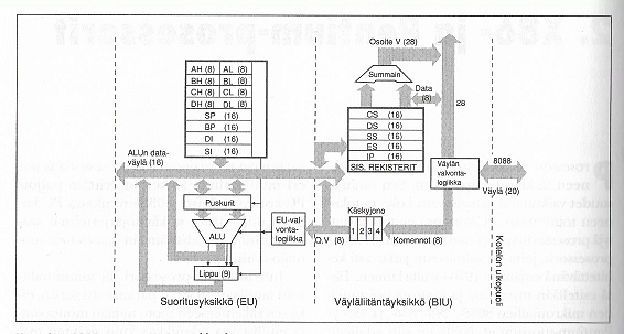
8088-prosessorissa (8-bittinen arkkitehtuuri) on sisäinen neljän käskyn mittainen käskyjono, josta käskyt siirretään sekventiaalisesti suoritettavaksi. Tällä tekniikalla pystytään vähentämään hitaita muistiosoituksia.
80286-prosessorissa (8/16-bittinen arkkitehtuuri) sisäiseen käskyjonoon haetaan automaattisesti aina 2-3 käskyä kerrallaan. Käskyt suoritetaan sekventiaalisesti. Jos haettu käsky on hyppykäsky, hylätään jono ja täytetään se uudelleen hyppykäskyn osoittamasta paikasta.
80386-prosessoreissa (32-bittinen arkkitehtuuri) toteutus perustui kaksivaiheeseen liukuhihnaan, eli seuraava käsky haetaan kun nykyistä ollaan suorittamassa. Hyppykäskyissä haettu seuraava käsky voidaan hylätä.
80486-prosessoreissa (32-bittinen arkkitehtuuri) yhden käskyn suorituksessa kuluu neljä kellojaksoa: käskyn nouto muistista, käskyn tulkitseminen (decode), operandin nouto muistista ja suoritus (execute). 486:sen liukuhihnassa taas on viisi vaihetta: käskyn nouto, käskyn tulkitseminen, muistiosoitteiden muodostus, suoritus ja takaisinkirjoitus (write back). 486:sessa oli myös suorittimeen integroitu matematiikkaprosessori liukulukulaskentaan, kun aiemmissa prosessorimalleissa se oli erillinen piiri samalla piirikortilla.
Pentium-prosessoreissa (alunperin 32-bittinen arkkitehtuuri) liukuhihnassa on viisi vaihetta, kuten 486:sessa. Pentium on itseasiassa superskalaaritekniikalla (tästä myöhemmin lisää..) toimiva prosessori, jolloin siinä on useita erillisiä mutta rinnakkaisia suoritusjonoja ja ALUja. Pentiumeissa on kaksi ALUa kokonaislukulaskentaan, joista toinen suoritti yksinkertaisia käskyjä (V-linja) ja toinen (U-linja) suoritti kaikkia käskyjä. Pentiumeissa on lisäksi liukulukulaskentaan oma matematiikkasuoritin, jolla on oma liukuhihna. Näin ollen Pentiumissa itseasiassa on kolme eri tavoin liukuhihnoitettua ALUa!

Lopuksi
Liukuhihnatoteutuksista on siis merkittävästi hyötyä suorittimen suorituskyvylle, mutta hintana on yksittäisen käskyn suoritusajan piteneminen ja vaativampi mikroarkkitehtuurin toteutus.
Oikeissa suorittimissa (M)IPS ei ole kovin hyvä mittari suoritusteholle, koska se ilmoittaa parhaan mahdollisen tuloksen ja oikeita ohjelmia suorittaessa IPS vaihtelee. Eli keskimääräisesti se on jotain muuta kuin paras mahdollinen. Suorituskykyä tarkastelemme vielä lisää myöhemmässä materiaalissa.
Anna palautetta
Kommentteja materiaalista?